text (R)

Overview

The R text package wraps transformer language models, such as BERT, for psychological and behavioral text analysis. It embeds text, trains models on top of embeddings, and visualizes how words relate to numeric outcome variables. This tutorial reproduces the Supervised Dimension Projection (SDP) workflow from the package’s Psychological Methods tutorial.

We apply this workflow to a synthetic ChatbotLab corpus of 19 person-to-AI conversations. Each “person” speaker is tagged with age, gender, persona, and a PHQ-9 depression-severity score. Supervised Dimension Projection places individual words along a continuous variable. Here, that variable is PHQ-9.

Data Format

textEmbed() and textProjection() expect a flat data frame. Each row is one text unit, such as one participant, with a text column and numeric covariate columns aligned to it.

This repository provides that shape in conversation_data/text/:

conversation_data/text/
  msgs.csv         # message_id, user_id, timestamp, message
  outcomes.csv     # user_id, age, gender, persona, phq9

Only “person” utterances are included. The assistant has no outcome variables attached to it. conversation_data/to_dlatk_format.py generates these files.

Setup

install.packages("text")
library(text)

# One-time: creates a Python environment with torch and transformers
textrpp_install()
textrpp_initialize()

Loading and Preparing the Data

textProjection needs one row per participant: their full conversation text alongside their PHQ-9 score. Join the messages to the outcomes table and collapse each participant’s messages, in timestamp order, into a single string:

library(dplyr)
library(readr)

msgs <- read_csv("conversation_data/text/msgs.csv")
outcomes <- read_csv("conversation_data/text/outcomes.csv")

person_data <- msgs %>%
  arrange(user_id, timestamp) %>%
  group_by(user_id) %>%
  summarise(text = paste(message, collapse = " ")) %>%
  inner_join(outcomes, by = "user_id")

This gives a 19-row data frame. Each row is one participant, with a text column holding their full conversation, and their phq9, age, gender, and persona.

Embedding the Text

word_embeddings <- textEmbed(
  person_data$text,
  model = "bert-base-uncased",
  aggregation_from_tokens_to_word_types = "mean",
  keep_token_embeddings = FALSE
)

word_embeddings$texts$texts holds one BERT embedding per participant, mean-aggregated across their tokens. word_embeddings$word_types$texts holds one decontextualized embedding per unique word type across the whole corpus. textProjection requires both.

Supervised Dimension Projection

projection_results <- textProjection(
  words = person_data$text,
  word_embeddings = word_embeddings$texts$texts,
  word_types_embeddings = word_embeddings$word_types$texts,
  x = person_data$phq9,
  split = "mean",
  min_freq_words_test = 2
)

With only 19 participants, a mean split is more stable than the package’s default quartile split. This puts 10 participants above the mean PHQ-9 of 11.6, and 9 at or below it. min_freq_words_test = 2 drops words that occur only once. Otherwise, these rare words would dominate the extremes on a corpus this small.

Plotting

plot_n_words_middle controls how many words near the center of the PHQ-9 dimension get labeled, in addition to the extremes. The default is a sparse plot; raising it (here, to 8) surfaces more of the mid-range vocabulary.

Font sizes for axis text/titles and the legend aren’t exposed as textProjectionPlot() arguments, and $final_plot is a cowplot::ggdraw() composite, so adding + theme(...) to it afterward has no effect — the inner scatter plot is already baked into a grob by the time it’s returned. To restyle it, intercept the package’s internal (unexported) plotting function with trace() to capture the scatter plot before it’s composited, apply the theme there, then re-render:

trace(text:::textPlotting, exit = quote({
  assign("captured_plot", returnValue(), envir = .GlobalEnv)
}), print = FALSE, where = asNamespace("text"))

plot_projection <- textProjectionPlot(
  word_data = projection_results,
  min_freq_words_plot = 2,
  plot_n_word_extreme = 8,
  plot_n_word_frequency = 4,
  plot_n_words_middle = 8,
  y_axes = FALSE,
  p_alpha = 1,
  title_top = "",
  x_axes_label = "Low vs. High PHQ-9 score",
  p_adjust_method = "none",
  word_size_range = c(12, 30)
)

untrace(text:::textPlotting, where = asNamespace("text"))

captured_plot + ggplot2::theme(
  axis.text = ggplot2::element_text(size = 40),
  axis.title = ggplot2::element_text(size = 34),
  plot.title = ggplot2::element_blank(),
  legend.position = "none"
)

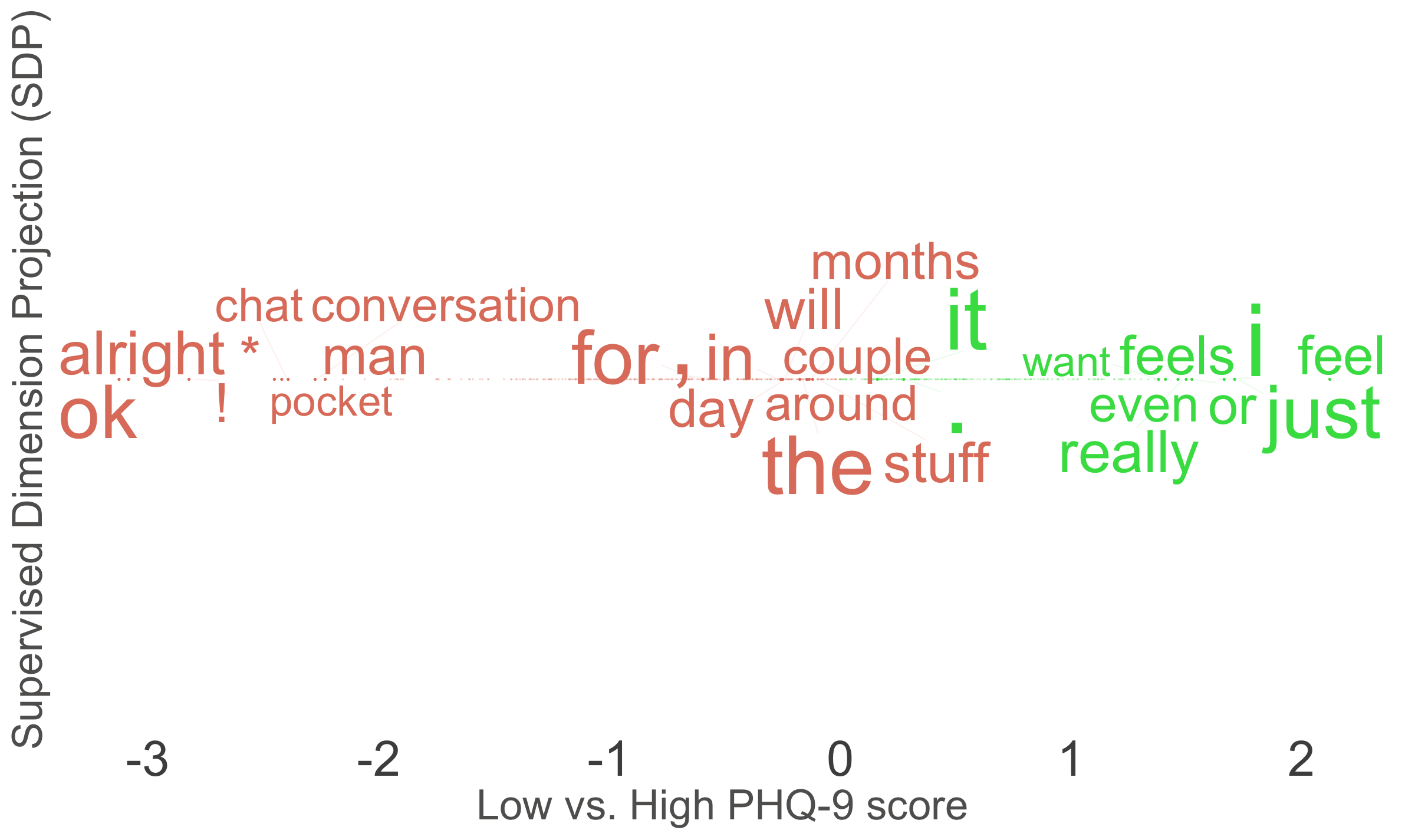
Each point is a word type positioned along the PHQ-9 dimension on the x-axis. Setting y_axes = FALSE keeps this to the one-dimensional case, since we project onto only one variable. Point size scales with word frequency, though we drop the legend that normally decodes that (and the plot title) to keep the enlarged-font version above readable. The most extreme and most frequent words on each side are labeled.

Results

Top words toward higher PHQ-9, by Supervised Dimension Projection score:

word	n	SDP	Cohen’s d	p
feel	17	2.12	2.18	.054
just	98	1.71	1.72	.111
i	325	1.66	1.67	.114
or	16	1.52	1.51	.164
feels	17	1.50	1.48	.182
really	28	1.46	1.44	.207
even	9	1.41	1.38	.237

Top words toward lower PHQ-9:

word	n	SDP	Cohen’s d	p
alright	36	-3.13	-3.70	< .001
ok	99	-3.08	-3.65	< .001
!	16	-2.82	-3.36	< .001
chat	4	-2.42	-2.91	.007
conversation	5	-2.28	-2.75	.018
man	16	-2.23	-2.70	.019

Higher-PHQ-9 words include affect and hedging language, such as feel, feels, and just. Lower-PHQ-9 words include upbeat, closing language, such as alright, ok, and man. Only the lower-PHQ-9 words clear p < .05, uncorrected.

With only 19 participants, this is a demonstration of the workflow, not a finding. Treat the plot and tables as a template. Re-run this code on a properly powered study export, and set p_adjust_method to something other than "none".

Generalizing

Swap phq9 for any other outcome column in outcomes.csv: age, a REDCap or Qualtrics field passed through at Survey Integration, or a score from your own instrument. The rest of the pipeline stays the same: textEmbed, then textProjection, then textProjectionPlot. The same embeddings also feed textTrain and textPredict, if you want a predictive model instead of a projection plot.